Work performed under contract to PE Applied Biosystems, Inc. United States Patent 6,131,072
Bioinformatics 2001 & 2002 Readers’ Choice Award Winner: Sequencing Analysis Software
Electrophoretic Gel Image Tracking by the Simulated Annealing of Splines Augmented by Local Error Estimates
Abstract
Introduction
Global Optimization for Tracking
Tracker Initialization
Tracking by Simulated Annealing
Peak Constraint Error
Lane Spacing Constraint Error
Regularity Constraint Errors
Generation Function
Local Temperature Control
Results
Conclusions
References
Software has been developed to automatically track lanes in four-color fluorescence-based, electrophoretic gel images created for DNA sequencing and fragment analysis. Lanes are modeled using splines. A simulated annealing based algorithm adjusts the splines to yield a proper tracking. Local error estimates are used to focus the attention of the system on poorly tracked areas and allow the algorithm to be greedy in well-tracked areas yielding an efficient and effective algorithm.
Keywords: Lane, Tracking, Gel, Image, Electrophoresis, Simulated annealing, Local error
Gel electrophoresis is used to sort DNA fragments by size by virtue of causing smaller DNA fragments to migrate through the gel faster then larger ones [1]. An imaging process measures the concentration of the migrating electrophoresed DNA fragments producing an image where the vertical scan-axis has increasing fragment sizes through time (Figure 1). Like-sized and therefore co-migrating fragments produce compact high concentrations of DNA fragments that appear as bands in the image. Different samples, each containing multiple DNA fragments, are loaded in individual wells at one end of the gel (across the channel-axis) and electrophoresed simultaneously. The trajectory of the DNA fragments for each sample, as it appears in the image, is known as a lane. The tracking algorithm determines, from the image, which bands came from which lane, and hence, which sample.
Two common applications of gel electrophoresis are DNA sequencing and DNA fragment analysis. A DNA fragment, or oligonucleotide, is a sequence of four different nucleotides as denoted by the letters C, A, T, and G. DNA sequencing determines the sequence of nucleotides (e.g. CATTG) that comprise a given section of DNA. The fragments of each sample well consist of all possible partial copies of a DNA (e.g. C, CA, CAT, CATT, CATTG). By labeling the last nucleotide in each sub-sequence with a different color and electrophoresing a sample’s fragments in the same lane, the complete sequence can be deduced (Figure 1, left). In fragment analysis, only certain sized fragments are synthesized, producing sparse images (Figure 1, right).
There is nothing that explicitly links one band of a lane to any other bands in that lane. Linking the bands of a lane may be particularly difficult when the lane is highly curved and consists of disparate bands. Furthermore, it may be difficult to detect each band or the center of each band due to noise, interaction with other bands, and chemistry related issues. These facts make it impossible to create a deterministic trivial method to link all the bands of each sample together into lanes. Historically, this has been a difficult problem to solve, especially with fragment analysis gels. Time consuming human intervention was usually necessary to clean up the tracking.
Global Optimization for Tracking
Various tracking algorithms already exist [2,3]. Most don’t attempt fragment analysis because of the scarcity of bands. Generally, these algorithms perform tracking on one small region of the gel at a time. This limited context combined with the lack of feedback to diffuse non-local information often yields poor results in areas of scarce or problematic data.
It is not possible to construct lanes from peaks alone in areas of scarce and perhaps imperfect peaks. However, when combined with the estimated positions and shapes of all the lanes, a priori lane spacing information, and regularity constraints, an effective error metric can be devised that corresponds well to the relative merit of a configuration of lanes.
The applicability and effectiveness of an error metric combined with the need for global information make an optimization approach a logical choice. Simulated annealing has been chosen for the optimization because it does not require the explicit creation of a gradient and furthermore provides the benefit of global optimization. (Note, a BFGS Quasi-Newton local optimization did not yield very good results.) To expedite the algorithm, several features have been added to the standard simulated annealing algorithm. These features make use of the properties specific to the tracking problem. One of these properties is the ability to obtain a gross estimate of the tracking error for a local region. The local estimate is certainly insufficient for optimization (otherwise the region by region approach described above would be adequate) but is generally sufficient to indicate regions of the system that are extremely bad or good. This information is used to bias the attention and efforts of the simulated annealing algorithm in proportion to the local error estimates.
The algorithm described in this paper is one part of a complete tracking system. Previous to this algorithm, another process accurately finds the center points of the bands. The one-dimensional profile of a band’s intersection with a center of a lane is typically called a peak. However, for the purposes of this paper "peak" will refer to the estimated center point of a band. For computational expediency, a binary "peak image" is formed from the output peaks by compression in the scan axis. This is feasible because the peaks are relatively sparse and lane curvature typically very small except for the lower scans (i.e. the "primer peak" area).
Since gel electrophoresis naturally produces smooth slowly changing lane shapes, splines are an appropriate way to model lanes. Moving the tie points that define a spline defines a new trajectory for the model lane as defined by the specific type of spline used. A spline’s flexibility can be matched to the requirements of the system by setting the density of its tie points.
The tracker specifically uses Catmull-Rom (Catmull) splines. Catmull splines smoothly interpolate through their tie points and have the property that the tangent to the spline at one tie point has the same slope as the line which connects both that tie point’s neighboring tie points. The implementation uses evenly spaced tie points which simplifies the computation. The tie points occur at the same scans coordinates in all the lanes, i.e. tie point t (the tth tie point) in model lane l has the same scan coordinate as any other lane’s tie point t. Catmull tie points require four consecutive tie points to define the spline segment that occurs between the second and third of those tie points.
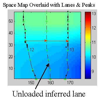
As mentioned above, each lane corresponds to a well. Sometimes, no sample is loaded in a well and so the number of loaded lanes, i.e. the number of lanes shown in the image, is unknown. In order for the tracker algorithm described herein to work effectively, it is necessary to determine the number of loaded lanes and create a model lane in the vicinity of each lane (as represented in the peak image). This is accomplished by another tracker algorithm that determines the number of lanes and tracks those lanes but only for the center scans of the image where the lanes are typically less curved. The resulting model lanes are then extrapolated to all the scans of the peak image. The high curvature of the lanes in the extrapolated regions invariably yields model lanes that are essentially untracked and cross other lanes and so present a difficult tracking problem (Figure 2).
Tracking by Simulated Annealing
The concept of simulated annealing was introduced by Metropolis [4] for application to the problems of statistical mechanics as an extension to the Monte Carlo algorithm and was later applied to optimization [5,6]. The concept of simulated annealing is taken from nature where a slow cooling of a material will produce a particularly good crystallization, i.e. low energy state (whereas a fast cooling will produce poor crystallization). This corresponds to an optimization procedure reaching a (near) global minimum.
Here's a link to some basic algorithm info: Markov Chain Monte Carlo (MCMC)
The (standard) simulated annealing algorithm is modeled as a physical many-particle system progressing toward thermal equilibrium which will then conform to the Boltzmann-Gibbs distribution. The standard simulated annealing algorithm is as follows:
A state of the simulated annealing tracker, X, is defined by the tie points that specify the model lane splines. The generation function creates a trial state of the tracker, Xtrial, by moving the tie points of the current state in the channel-axis. The error (i.e. energy) of the trial state, E(Xtrial), is calculated by an error function that has been designed with the intent that lower error implies better tracking and perfect tracking is obtained at the global minimum. If the trial state is accepted by the acceptance function then it becomes the new state. The standard stochastic acceptance function,
where u(x) is a uniform variate in [0,1), accepts all trial states of lower error and an exponentially decreasing fraction of higher energy trial states as normalized by the current temperature, T. The tracker’s error function is constructed as the weighted average of several constraint errors. These constraint errors are described below.
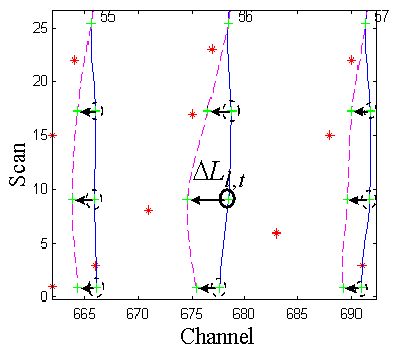
The primary constraint attempts to minimize the distance of all the peaks to the closest lanes. The distance from a peak to a model lane is taken to be the difference in the channel coordinates of the model lane and peak at the peak’s scan coordinate. The tracker, as currently implemented, assigns probability of peak ownership (i.e. that a peak is part of a lane as given by a particular model lane) to just the two model lanes that currently bound each peak. (Note that as the model lanes move the bounding lanes for any particular peak may change.) This may not be ideal but it appears to be sufficient and it is computationally inexpensive.
The formulation of peak error is based on the ad hoc concept that a peak’s error should be the squared distance with respect to both its bounding model lanes, each weighted by the estimated probability that the corresponding lane actually owns the peak. The probabilities are computed as relative distances of a peak to the two bounding lanes resulting in a formulation that is, mechanically, the linear interpolation of the two squared distances. Given a peak k bounded by two model lanes separated by D channels at the scan of peak k, and Dn and Dp the channel distances of peak k from the next and previous model lanes, respectively, then the peak constraint error for peak k, EPk, is as follows:
Given a fixed D and viewing Dp as potential peak channel locations between 0 and D, EPk describes a parabola with its maximum and 0 derivative, which can be interpreted as the point of least certainty of lane ownership, at D/2 and its roots at 0 and D. The extra divisor D is a normalization term that yields a derivative that approaches 1 on either side of Dp=0 regardless of the two distances that correspond to the lanes on either side of a model lane (i.e. at Dp=0). This attenuates the otherwise implicit bias in accepting transitions toward the side of the lane with the closest neighboring lane. The normalization furthermore reduces the growth of EPk with respect to D to linear rather then quadratic which increases transition flexibility for larger values of D.
The spacing constraint error, Es, measures the discrepancy between the actual and expected channel distance between consecutive model lanes as determined from the "space map." The space map itself is created with respect to the channel distances between consecutive peaks within each scan of the peak image. For each coordinate in the peak image, the space map gives the expected channel distance from a lane at that coordinate to the next possible lane (i.e. the lane that corresponds to the next well regardless of whether it was loaded or not).
Since lanes may be unloaded, consecutive model lanes may be separated by large distances that correspond to unloaded lanes between them. Therefore, the expected distance between model lanes must be derived by accumulating the expected lane distances for all the lanes that are thought to be between two consecutive model lanes. Computing the number of lanes between two model lanes is accomplished by repeatedly using the space map value to predict the position of the next lane from the last predicted lane until the next model lane is reached. This, however, is only sensible if the model lanes are properly spaced. This would seem to be a circular argument except for the fact that, as stated above, the lanes have already been tracked for the center portion of the image. Therefore, this approach can be used for the center tie points to estimate the number of lanes from one consecutive model lane to the next. Since the number of lanes to the next model lane must be the same for the entire lane, it can be used as the number of iterations to predict the position of the next model lane for any scan of the lane. The final iteration yields the expected position of the next model lane at a particular scan thereby yielding the expected distance between two model lanes (at that scan).
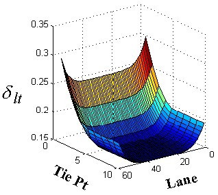
To expedite the computation, the spacing constraint error is determined only with respect to the tie points (not the scans between the tie points). The spacing error with respect to the tth tie point on lane l is as follows:
where SAlt and SElt are the actual and expected channel distances, respectively, between the tth tie point on model lanes l and l+1 and d lt is the tolerance that reflects the inaccuracy of the space map’s expected lane distance values. The tolerance is larger for the primer peak and outside lane tie points whose spacing is more irregular. The total spacing error, ES, is the sum squared tie point errors across all l and t.
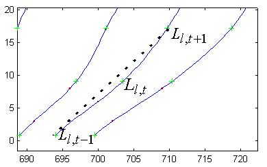
The lane similarity constraint error, EI, measures the difference in shape of consecutive model lanes. The computation is simplified by again using just the tie point channel coordinates. The error for each tie point, EIlt, as shown below, is just the modified difference of the change in channel coordinates of a consecutive pair of tie points in the next lane and the change in channel coordinates of the corresponding pair of tie points in the current lane:
where AIlt is an attenuation factor (a maximum value of 1) and Ll,t is the channel coordinate of the tth tie point of model lane l. The attenuation factor is less in areas of expected high curvature, the primer peak and outer lane areas, and varies inversely with model lane distance. The total lane similarity constraint error, EI, is the sum squared tie point similarity errors.
A new lane similarity constraint error based on linear interpolation has been implemented but not yet formally tested. The constraint is minimized when the slope of the line joining two tie points on a lane is the linear interpolation of the corresponding slopes on both of its neighboring lanes. The formulation is as follows:
where Nlj is the estimated number of lanes between the model lanes l and j and D Llt=Ll,t+1-Ll,t. Even for distant neighboring model lanes, i.e. large Nlj, as well as in the primer peak area, the shapes of lanes are typically very close to the interpolation shape. Therefore, the attenuation term, AIlt, can be very mild yielding a strong constraint in the primer peak area.
The curvature constraint error, EC, is currently satisfied by straight model lanes. The error must therefore be attenuated for the primer peak and outer lane areas where highly curved lanes are to be expected. The computation is based on the difference of the change in channel coordinates of a pair of tie points in a lane and the change in channel coordinates of the previous pair of tie points in the same lane:
where AClt is an attenuation factor that is less in areas of expected high curvature which includes the primer peak and outer lane areas The total curvature constraint error, EC, is the sum squared tie point curvature errors.
As mentioned above, the generation function is responsible for generating the trial states of the system which, for the tracker, corresponds to new channel positions of the tie points. The standard generation function creates a trial state by generating a |X| dimensional movement for the current state with respect to either a temperature-scaled Gaussian, or Cauchy distribution [7]:
Unfortunately, the standard generating functions did not yield a practical rate of convergence. To increase the rate of convergence, the tracker uses a generation function that takes advantage of the spatial coherency of the lanes to create states that are more likely to produce lower error and also concentrates the systems efforts to those tie points that seem to be in poorly tracked areas.
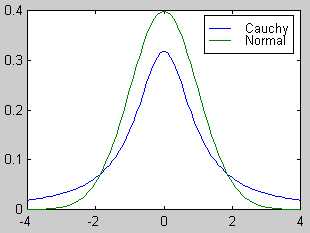
Rather then move all the tie points, the generation function applies the Cauchy generation function to just one selected tie point, i.e. a 1-dimensional Cauchy distribution, rather then to all the tie points (7) . In addition to the selected tie point, the tie points in a 2-d neighborhood around the selected tie point are also moved a fraction of the selected tie point’s movement. This movement is not done with respect to any formalism but rather based on the observation that the desired direction of movement for a tie point, especially at the start of tracking, tends to be the same as its neighbors. Furthermore, moving the neighboring tie points in the manner tends to better satisfy the regularity constraints.
The movement of the neighboring tie points is modeled as tension that relaxes with distance and over time. Relaxing the tension over time, implemented by factoring in the temperature T as a fraction of the initial temperature To, is appropriate given the decrease in correlation of the desired direction of movement for neighboring tie points as the system evolves. The movement of the neighboring tie points is:
where D Ll,t is the (channel) movement of the selected tie point and Nlj is the estimated number of lanes between the model lanes l and j. To accommodate the possibility of uncorrelated neighborhood tie point errors, the neighborhood radius is allowed to randomly vary between 0 and 3. The parameter u(x) is a uniform variate that increases state flexibility by allowing the system to more easily generate arbitrary states and a, a value between 0 and 1, regulates the amount of flexibility.
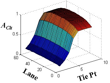
The choice of which tie point is selected each iteration is a stochastic process with respect to a probability density function, S, that is periodically computed over all tie points with respect to just the peak errors, EP (2). The probability assigned to each tie point is proportional to the total peak error attributed to the tie point. This biases the system to working on the portions of model lanes that are estimated to be poorly tracked.
The set of tie points affected by an individual peak error is taken to be all eight tie points that define the bounding spline segments of the respective peak. The magnitude of the affect to a tie point attributed to a peak error varies inversely with the distance of the affected tie point from the peak. The probability for selection of tie point (l, t) is as follows:
where Qlt = {pi | ![]() Ù
Ù ![]() } (i.e. peak pi has one of the
segments from model lane l that are located between tie points t-2 and t+2
as one of its bounding model lane segments), c(pi) and s(pi)
are the channel and scan coordinates of peak pi, respectively, D s(t) is the scan distance from any tie point t
to a neighboring one on the same lane, st(t) is the scan coordinate of
tie point t, EPpi is the peak error for peak pi,
Ll(s(pi)) is the channel coordinate of model lane l at
s(pi) and g(s(pi),D s(t),st(t))
is a normalized Gaussian centered at s(pi) with a standard deviation of D s(t) evaluated at st(t). The Gaussian
smears the error associated with a peak, EPpi, to all the tie points
that define the spline segments that bound the peak. The lower bound of d in the computation of S1lt, typically 0.3,
insures that some error is ascribed to each tie point which acts as insurance against the
significant probability that the local error estimate vastly underestimates the actual
error. The fact that EP is the only error constraint used makes the
technique somewhat fragile for areas of the peak image with very few peaks (where model
lanes that jump track may be still close to all peaks and so yield a small Ep).
However, testing seems to indicate that this is not a serious problem.
} (i.e. peak pi has one of the
segments from model lane l that are located between tie points t-2 and t+2
as one of its bounding model lane segments), c(pi) and s(pi)
are the channel and scan coordinates of peak pi, respectively, D s(t) is the scan distance from any tie point t
to a neighboring one on the same lane, st(t) is the scan coordinate of
tie point t, EPpi is the peak error for peak pi,
Ll(s(pi)) is the channel coordinate of model lane l at
s(pi) and g(s(pi),D s(t),st(t))
is a normalized Gaussian centered at s(pi) with a standard deviation of D s(t) evaluated at st(t). The Gaussian
smears the error associated with a peak, EPpi, to all the tie points
that define the spline segments that bound the peak. The lower bound of d in the computation of S1lt, typically 0.3,
insures that some error is ascribed to each tie point which acts as insurance against the
significant probability that the local error estimate vastly underestimates the actual
error. The fact that EP is the only error constraint used makes the
technique somewhat fragile for areas of the peak image with very few peaks (where model
lanes that jump track may be still close to all peaks and so yield a small Ep).
However, testing seems to indicate that this is not a serious problem.
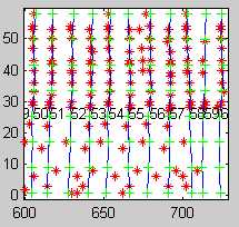
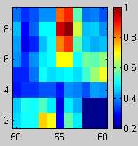
Initial S1lt
Initial Tracking
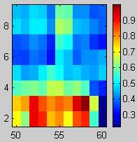
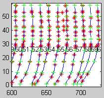
Final S1lt
Final Tracking
Periodically, taking advantage of the a priori assumption of lane shape similarity, the generation function changes model lanes that are estimated to be very poorly tracked to assume the shapes of neighboring lanes that are estimated to be extremely well tracked. This seems to be very effective in transitioning out of broad-based local minima (i.e. large regions of poor tracking).
To facilitate this, the tracker first uses peak error to generate two confidence values for each lane. One confidence value is created with respect to loose tolerances and the other with very tight tolerances. A tight tolerance confidence value is used to judge which lanes are good enough to be used to create shape templates for other close lanes. Reshaping lanes is a very drastic step and so only the best lanes can be allowed to affect an explicit change in another lane’s shape. A loose tolerance confidence value is used to judge whether a lane is so bad that bypassing the standard generation function is deemed expedient. The computation of a peak confidence for lane l, Cl, is as follows:
where Ql = {pi |![]() } (i.e. peak pi has model lane
l as one of its bounding model lanes), Dpi the distance of peak pi
to the closest lane, D the distance between the lanes that bound peak pi,
d 1 is a tolerance on the fraction of the
distance from the closest lane as compared to the total lane distance, and d 2 is a tolerance on the distance between the peak
and the closest lane. The tight and loose confidence values, CTl and CLl,
are generated by computing Cl with respect to smaller and larger
tolerance values of d 1 and d 2, respectively.
} (i.e. peak pi has model lane
l as one of its bounding model lanes), Dpi the distance of peak pi
to the closest lane, D the distance between the lanes that bound peak pi,
d 1 is a tolerance on the fraction of the
distance from the closest lane as compared to the total lane distance, and d 2 is a tolerance on the distance between the peak
and the closest lane. The tight and loose confidence values, CTl and CLl,
are generated by computing Cl with respect to smaller and larger
tolerance values of d 1 and d 2, respectively.
If model lane l is bad enough to warrant a shape change (a low value of CLl) and there exist two model lanes j and k on either side of l that are good enough to be used to create a template lane (high CTj and CTk) and are also sufficiently close (both within d lanes of l) then lane l is reshaped by a template lane created by a linear interpolation of model lanes j and k. Since interpolated lanes tend to be a very good estimate of actual lanes, it yields very effective shape modifications. A tie point of the interpolated template lane is formed as follows:
This is standard linear interpolation augmented with the template lane confidence values, CTk and CTj which act as additional modifiers to the lane distances Njl, and Nlk, respectively. The shape of lane l itself is formed as a confidence value weighted average of the interpolated template lane and lane l as follows:
Finally, the new lane l is determined by shifting the derived lane, Ml, such that its center tie point is its original center tie point:
where c is the index of the center tie point.
Inevitably, portions of model lanes will be well tracked while others will not. The tie points in such a region are close to their positions in the global minimum solution and so do not need the ability provided by simulated annealing to accept transitions to higher error. Accepting transitions to states of higher error when it is not needed will slow convergence and so given a fixed number of iterations will tend to result in a worse solution. This problem is mitigated by assigning a modifier to each tie point’s ability to accept transitions to higher error. The value of the modifier is based on the tie point’s estimated local error. A tie point’s modifier is applied when it is the generation function’s selected tie point.
The error metric must be very conservative lest it allow an incorrectly tracked area to be stuck in a local minimum due to the lack of ability to search for a global minimum by transitioning to higher error. Therefore, the system uses a variant of peak error that places stringent conditions on all peaks that effect each tie point. For each tie point there is a spatially local set of peaks, Qlt, used in the computation of its error. If none of those peaks violate the stringent conditions then it is assumed that the tie point is in a well-tracked area and so doesn’t require the acceptance of transitions to higher error (i.e. it can use the greedy algorithm). Otherwise, the standard simulated annealing acceptance (1) function is used. The modifier is determined as follows:
where Dpi, D, pi, d 1 and d 2 are as in (10). If Hlt is false the greedy algorithm is used.
An alternative to this discrete approach is to reduce the acceptance probability in a continuous way by using a separate temperature for each tie point in a manner similar to that used by J. Leinbach [8]. The temperature is set using a formula that is a small modification of Hlt:
where T0 is the initial maximum temperature of the system and Tlt is the prorated temperature associated with tie point (l,t). This approach is desirable because it can completely replace the a priori temperature schedule allowing dynamic temperature scaling of the generation distribution, acceptance, and tension functions by substituting Tlt, when tie point l,t is selected, for T in (7) , (1), and (8) respectively. Unfortunately, for reasons not yet understood, the continuous approach did not work as well as the discrete approach (in an informal test). Specifically, smaller errors were less prevalent while significant errors were more prevalent. Perhaps a non-linear function of Tlt would be more effective.
Table 1. Performance Statistics1
Fragment Analysis |
DNA Sequencing4 |
|
| Loaded lanes detected. | 97.6% |
98.5% |
| Lanes accurately tracked.5 - Lenient criteria 2 | 96.2% |
98.3% |
| Lanes accurately tracked.5 - Stringent Criteria 3 | 95.8% |
98.2% |
1
Fragment Analysis 3723 lanes from 87 gels; Sequence Analysis 11226 lanes from 148 gels, with valid multi-componenting. 2 Lanes touch bands. 3 Lanes go through the center of the bands. 4Statatistics for 388 channel only. 5Including undetected lanes.This tracking algorithm has helped to successfully automate the difficult task of tracking for fragment analysis, as well as DNA sequencing, providing robust and accurate tracking. While standard simulated annealing and local optimization almost always produced poor tracking, even after running many hours and even though they used the same error function, the described algorithm consistently produced excellent tracking in 1 to 2 minutes (for fragment analysis gels) on a Power Macintosh 225. The neighborhood tension generation function technique may be applicable to other problems for which spatial coherency is inherent. Dynamic attention focusing (9) and local temperature control, (14) or (15) , may be applicable to other problems for which local error can be estimated.
[1] L.M. Smith, J. Z. Sanders, R.J. Kaiser, P. Hughes, C. Dodd, C.R. Connell, C. Heiner, S.B.H. Kent, L.E. Hood, Fluorescence detection in automated DNA sequence analysis, Nature, 321, 1986, 674-678
[2] S. Millership, K. Ragoonaden, Automated Lane Detection and Comparison of Bacterial Electrophoretic Protein Fingerprints Using Fast Fourier Transformation, Computers and Biomedical Research, 25(4), Aug. 1992, 392-406
[3] Mathew L. Cooper, David R. Maffitt, Jeremy D. Parsons, LaDeana Hillier, David J. States, Lane Tracking Software for Four-color Fluorescence-based Electrophoretic Gel Images, Genomic Research, Nov. 1996, 1110-1117.
[4] M. Metropolis, A. Rosenbluth, M. Rosenbluth, A.Teller and E.Teller, Equation of State Calculations by Fast Computing Machines, J. Chem. Phys. 21, 1953, 1087-1092.
[5] S. Kirkpatrick, C.D. Gelatt Jr., M.P. Vecchi, Optimization by Simulated Annealing, Science, 220, 1983, 671-680.
[6] V. Cerny, Thermodynamical Approach to the Traveling Salesman Problem: An Efficient Simulation Algorithm, J. of Optimization Theory and App., 45(1), 1985, 41-51
[7] H. Szu and R. Hartley, Fast Simulated Annealing, Physics Letters A, 122(3,4), 1987, 157-162.
[8] D. Touretzky, Advances in Neural Information Processing Systems 1 (San Mateo CA; Morgan Kaufmann Publishers, Inc., 1989), 602-609